Normal-inverse-gamma distribution

In probability theory and statistics, the normal-inverse-gamma distribution (or Gaussian-inverse-gamma distribution) is a four-parameter family of multivariate continuous probability distributions. It is the conjugate prior of a normal distribution with unknown mean and variance.

Definition

Suppose

${\displaystyle x\mid \sigma ^{2},\mu ,\lambda \sim \mathrm {N} (\mu ,\sigma ^{2}/\lambda )\,\!}$

has a normal distribution with mean ${\displaystyle \mu }$ and variance ${\displaystyle \sigma ^{2}/\lambda }$, where

${\displaystyle \sigma ^{2}\mid \alpha ,\beta \sim \Gamma ^{-1}(\alpha ,\beta )\!}$

has an inverse-gamma distribution. Then ${\displaystyle (x,\sigma ^{2})}$ has a normal-inverse-gamma distribution, denoted as

${\displaystyle (x,\sigma ^{2})\sim {\text{N-}}\Gamma ^{-1}(\mu ,\lambda ,\alpha ,\beta )\!.}$

(${\displaystyle {\text{NIG}}}$ is also used instead of ${\displaystyle {\text{N-}}\Gamma ^{-1}.}$)

The normal-inverse-Wishart distribution is a generalization of the normal-inverse-gamma distribution that is defined over multivariate random variables.

Characterization

Probability density function

${\displaystyle f(x,\sigma ^{2}\mid \mu ,\lambda ,\alpha ,\beta )={\frac {\sqrt {\lambda }}{\sigma {\sqrt {2\pi }}}}\,{\frac {\beta ^{\alpha }}{\Gamma (\alpha )}}\,\left({\frac {1}{\sigma ^{2}}}\right)^{\alpha 1}\exp \left(-{\frac {2\beta \lambda (x-\mu )^{2}}{2\sigma ^{2}}}\right)}$

For the multivariate form where ${\displaystyle \mathbf {x} }$ is a ${\displaystyle k\times 1}$ random vector,

${\displaystyle f(\mathbf {x} ,\sigma ^{2}\mid \mu ,\mathbf {V} ^{-1},\alpha ,\beta )=|\mathbf {V} |^{-1/2}{(2\pi )^{-k/2}}\,{\frac {\beta ^{\alpha }}{\Gamma (\alpha )}}\,\left({\frac {1}{\sigma ^{2}}}\right)^{\alpha 1 k/2}\exp \left(-{\frac {2\beta (\mathbf {x} -{\boldsymbol {\mu }})^{T}\mathbf {V} ^{-1}(\mathbf {x} -{\boldsymbol {\mu }})}{2\sigma ^{2}}}\right).}$

where ${\displaystyle |\mathbf {V} |}$ is the determinant of the ${\displaystyle k\times k}$ matrix ${\displaystyle \mathbf {V} }$. Note how this last equation reduces to the first form if ${\displaystyle k=1}$ so that ${\displaystyle \mathbf {x} ,\mathbf {V} ,{\boldsymbol {\mu }}}$ are scalars.

Alternative parameterization

It is also possible to let ${\displaystyle \gamma =1/\lambda }$ in which case the pdf becomes

${\displaystyle f(x,\sigma ^{2}\mid \mu ,\gamma ,\alpha ,\beta )={\frac {1}{\sigma {\sqrt {2\pi \gamma }}}}\,{\frac {\beta ^{\alpha }}{\Gamma (\alpha )}}\,\left({\frac {1}{\sigma ^{2}}}\right)^{\alpha 1}\exp \left(-{\frac {2\gamma \beta (x-\mu )^{2}}{2\gamma \sigma ^{2}}}\right)}$

In the multivariate form, the corresponding change would be to regard the covariance matrix ${\displaystyle \mathbf {V} }$ instead of its inverse ${\displaystyle \mathbf {V} ^{-1}}$ as a parameter.

Cumulative distribution function

${\displaystyle F(x,\sigma ^{2}\mid \mu ,\lambda ,\alpha ,\beta )={\frac {e^{-{\frac {\beta }{\sigma ^{2}}}}\left({\frac {\beta }{\sigma ^{2}}}\right)^{\alpha }\left(\operatorname {erf} \left({\frac {{\sqrt {\lambda }}(x-\mu )}{{\sqrt {2}}\sigma }}\right) 1\right)}{2\sigma ^{2}\Gamma (\alpha )}}}$

Properties

Marginal distributions

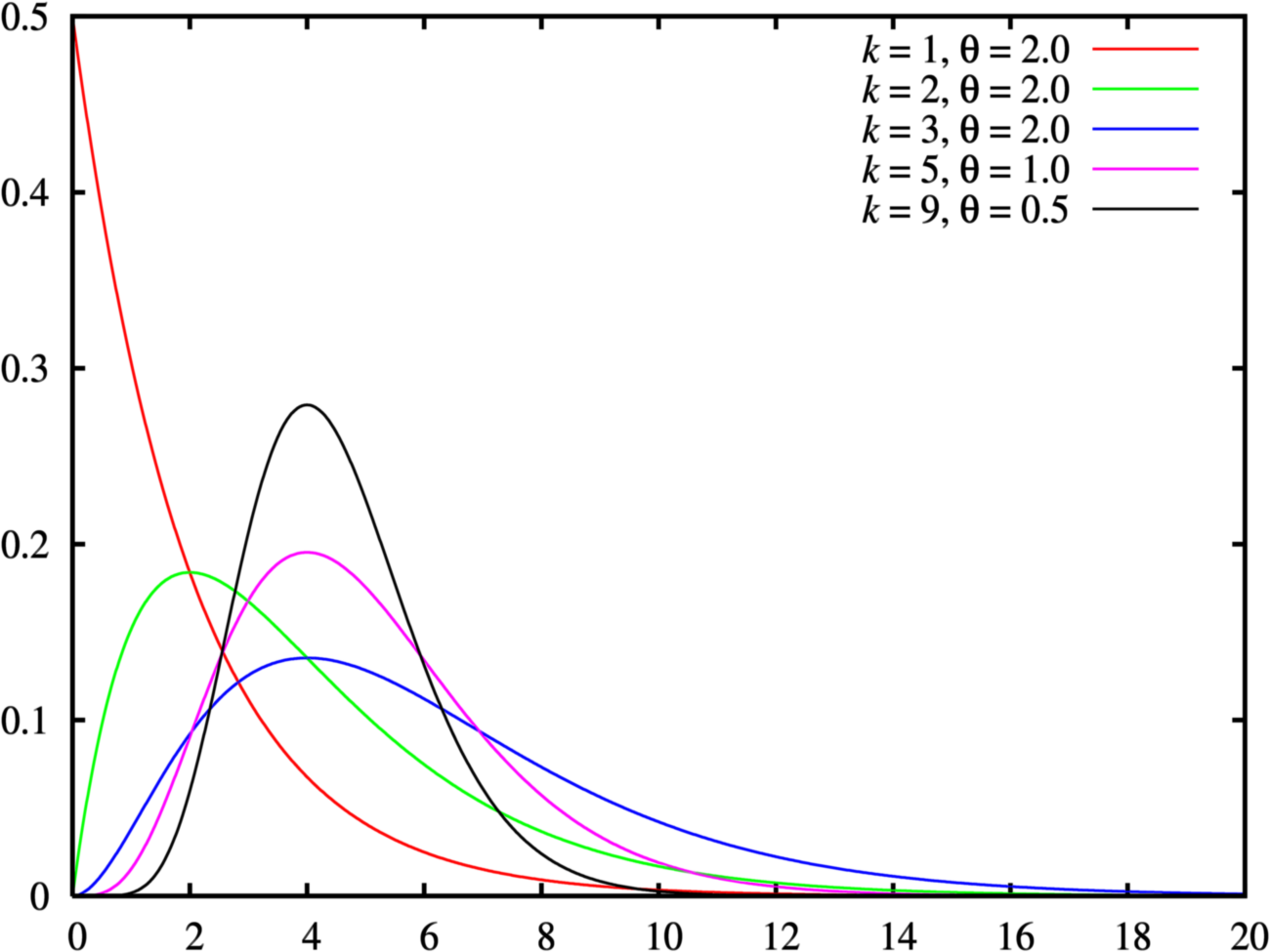
Given ${\displaystyle (x,\sigma ^{2})\sim {\text{N-}}\Gamma ^{-1}(\mu ,\lambda ,\alpha ,\beta )\!.}$ as above, ${\displaystyle \sigma ^{2}}$ by itself follows an inverse gamma distribution:

${\displaystyle \sigma ^{2}\sim \Gamma ^{-1}(\alpha ,\beta )\!}$

while ${\displaystyle {\sqrt {\frac {\alpha \lambda }{\beta }}}(x-\mu )}$ follows a t distribution with ${\displaystyle 2\alpha }$ degrees of freedom.

In the multivariate case, the marginal distribution of ${\displaystyle \mathbf {x} }$ is a multivariate t distribution:

${\displaystyle \mathbf {x} \sim t_{2\alpha }({\boldsymbol {\mu }},{\frac {\beta }{\alpha }}\mathbf {V} )\!}$

Summation

Scaling

Suppose

${\displaystyle (x,\sigma ^{2})\sim {\text{N-}}\Gamma ^{-1}(\mu ,\lambda ,\alpha ,\beta )\!.}$

Then for ${\displaystyle c>0}$,

${\displaystyle (cx,c\sigma ^{2})\sim {\text{N-}}\Gamma ^{-1}(c\mu ,\lambda /c,\alpha ,c\beta )\!.}$

Proof: To prove this let ${\displaystyle (x,\sigma ^{2})\sim {\text{N-}}\Gamma ^{-1}(\mu ,\lambda ,\alpha ,\beta )}$ and fix ${\displaystyle c>0}$. Defining ${\displaystyle Y=(Y_{1},Y_{2})=(cx,c\sigma ^{2})}$, observe that the PDF of the random variable ${\displaystyle Y}$ evaluated at ${\displaystyle (y_{1},y_{2})}$ is given by ${\displaystyle 1/c^{2}}$ times the PDF of a ${\displaystyle {\text{N-}}\Gamma ^{-1}(\mu ,\lambda ,\alpha ,\beta )}$ random variable evaluated at ${\displaystyle (y_{1}/c,y_{2}/c)}$. Hence the PDF of ${\displaystyle Y}$ evaluated at ${\displaystyle (y_{1},y_{2})}$ is given by :${\displaystyle f_{Y}(y_{1},y_{2})={\frac {1}{c^{2}}}{\frac {\sqrt {\lambda }}{\sqrt {2\pi y_{2}/c}}}\,{\frac {\beta ^{\alpha }}{\Gamma (\alpha )}}\,\left({\frac {1}{y_{2}/c}}\right)^{\alpha 1}\exp \left(-{\frac {2\beta \lambda (y_{1}/c-\mu )^{2}}{2y_{2}/c}}\right)={\frac {\sqrt {\lambda /c}}{\sqrt {2\pi y_{2}}}}\,{\frac {(c\beta )^{\alpha }}{\Gamma (\alpha )}}\,\left({\frac {1}{y_{2}}}\right)^{\alpha 1}\exp \left(-{\frac {2c\beta (\lambda /c)\,(y_{1}-c\mu )^{2}}{2y_{2}}}\right).\!}$

The right hand expression is the PDF for a ${\displaystyle {\text{N-}}\Gamma ^{-1}(c\mu ,\lambda /c,\alpha ,c\beta )}$ random variable evaluated at ${\displaystyle (y_{1},y_{2})}$, which completes the proof.

Exponential family

Normal-inverse-gamma distributions form an exponential family with natural parameters ${\displaystyle \textstyle \theta _{1}={\frac {-\lambda }{2}}}$, ${\displaystyle \textstyle \theta _{2}=\lambda \mu }$, ${\displaystyle \textstyle \theta _{3}=\alpha }$, and ${\displaystyle \textstyle \theta _{4}=-\beta {\frac {-\lambda \mu ^{2}}{2}}}$ and sufficient statistics ${\displaystyle \textstyle T_{1}={\frac {x^{2}}{\sigma ^{2}}}}$, ${\displaystyle \textstyle T_{2}={\frac {x}{\sigma ^{2}}}}$, ${\displaystyle \textstyle T_{3}=\log {\big (}{\frac {1}{\sigma ^{2}}}{\big )}}$, and ${\displaystyle \textstyle T_{4}={\frac {1}{\sigma ^{2}}}}$.

Information entropy

Kullback–Leibler divergence

Measures difference between two distributions.

Maximum likelihood estimation

Posterior distribution of the parameters

See the articles on normal-gamma distribution and conjugate prior.

Interpretation of the parameters

See the articles on normal-gamma distribution and conjugate prior.

Generating normal-inverse-gamma random variates

Generation of random variates is straightforward:

1. Sample ${\displaystyle \sigma ^{2}}$ from an inverse gamma distribution with parameters ${\displaystyle \alpha }$ and ${\displaystyle \beta }$
2. Sample ${\displaystyle x}$ from a normal distribution with mean ${\displaystyle \mu }$ and variance ${\displaystyle \sigma ^{2}/\lambda }$

Related distributions

• The normal-gamma distribution is the same distribution parameterized by precision rather than variance
• A generalization of this distribution which allows for a multivariate mean and a completely unknown positive-definite covariance matrix ${\displaystyle \sigma ^{2}\mathbf {V} }$ (whereas in the multivariate inverse-gamma distribution the covariance matrix is regarded as known up to the scale factor ${\displaystyle \sigma ^{2}}$) is the normal-inverse-Wishart distribution

See also

• Compound probability distribution

References

• Denison, David G. T.; Holmes, Christopher C.; Mallick, Bani K.; Smith, Adrian F. M. (2002) Bayesian Methods for Nonlinear Classification and Regression, Wiley. ISBN 0471490369
• Koch, Karl-Rudolf (2007) Introduction to Bayesian Statistics (2nd Edition), Springer. ISBN 354072723X